Raman microscope operation and first results.
|
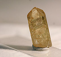
An example of Raman spectrum obtained with the instrument described in
previous pages is reproduced below. An apatite single crystal (picture
on the right) has been used as a target to get this spectrum. The CCD image
shows a series of faint Raman lines. The laser line which should appear
to the left of the image has been nearly eliminated by the beam splitter
and blocking filter and is barely visible in the picture.
|
|
|
Raman spectrum of apatite single crystal from CCD camera.
Figure 1
|
|
|
|
|
To convert the CCD image to a spectral curve, I have used Visual Spec, the freeware from Valérie Desnoux http://astrosurf.com/vdesnoux/ . This software written for data processing of astronomical spectra can also been used for Raman spectroscopy image conversion and for spectral calibration with neon light to get a wavelength x-scale in nanometers. The raw spectra reported on this page illustrate the first steps in the Raman spectra processing : image conversion to spectrum and spectral calibration. Generally, the Raman spectra appear above a more or less intense continuous background which must be subtracted from the spectrum. As usually done in vibrational spectroscopy, the wavelength scale is converted from wavelength in nanometers to wave numbers in cm-1. These two additional processings of spectra will be explained later. The spectrum reproduced in figure 2 was obtained with the dichroic plate beam splitter in place. The laser line peak in the spectrum is very low compared to the Raman intensity due to the 2 steps removals of direct laser light. The combined absorption of both filters can be seen in figure 2 between 637 and 640 nm.
|
|
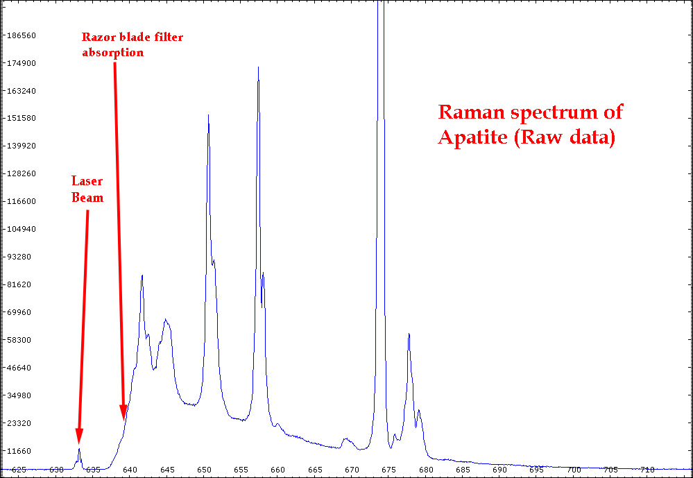
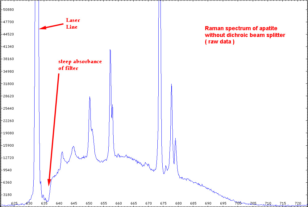 Figure 3
|
|
|
The spectrum of figure 3 has been recorded with a traditional beam splitter (50-50). It means that 50 % of the light is lost on each pass through the splitter. In the spectrum we can see that the laser intensity is now very high which is a problem when recording very weak Raman spectra like pyrite for instance due to spurious reflections inside the spectrograph. Comparing figure 2 and 3, it can be seen that the background is much more noisy in figure 3 obtained with a traditional beam splitter ( much less expensive). This is due to the light loss of this splitter in comparison with the dichroic mirror. I can also be noticed in those figures that the steepness of the absorption at 635-640 nm is much higher if the laser rejection filter is used alone. A small part of the spectrum is thus lost if the dichroic mirror and laser rejection filter are used together. However due to the higher intensity, the accumulation time for detection is much reduced when both filtering devices are used. The shape of the background in figure 3 requires further comments. This background curve is approximately bell shaped. This is a consequence of the vignetting of the spectrograph already mentioned previously. From that curve it can be inferred that the sensitivity of the Raman signal is wavelength dependant. At 700 nm (1500cm-1) the intensity of the signal is close to zero; the CCD is not fully covered by the spectrum. The spectrum presented here were recorded at a H20 wavelength of 670nm. Of course it is always possible to change that position to record spectra at higher wavelengths. The sensitivity variation with wavelength must be taken into account when comparing to literature spectra.
|
|
Neon spectrum from CCD camera
Figure 4 |
|
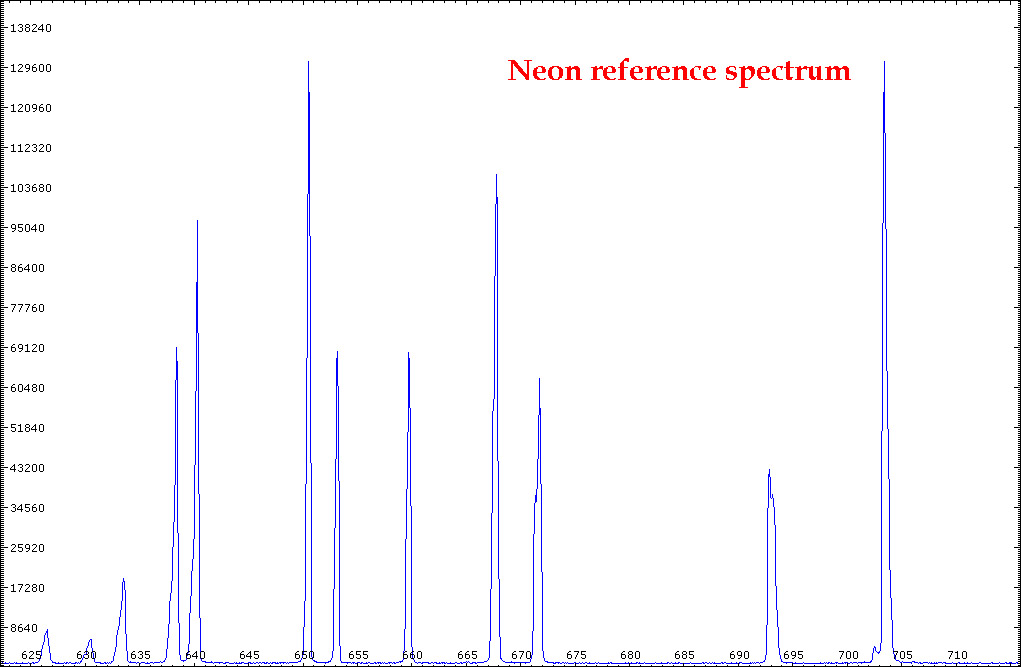 Figure 5
|
|
|
The wavelength calibration of the Raman spectra is made by comparing the raw Raman curve with a known line spectrum of a neon bulb. After each recording of the Raman data, the top flip mirror is rotated so that the neon light can reach the spectrograph. An example of such a neon spectrum on the CCD is reproduced in figure 4. This image is converted to spectrum in the usual way with the V Spec program. On the image, the imperfections of the H20 used as a spectrograph are obvious. As the grating is spherical, the aberrations are not fully corrected and a neon emission line appears somewhat curved. Due to field curvature, it is not possible to bring each part of the spectrum in perfect focus; a compromise should be found. For our calibration purpose, only the central horizontal part of the image where the lines are narrower is used. This procedure gives the spectrum in figure 5 without too much line broadening.
|
|
|
Figure 6 Final spectrum.
|
|
|
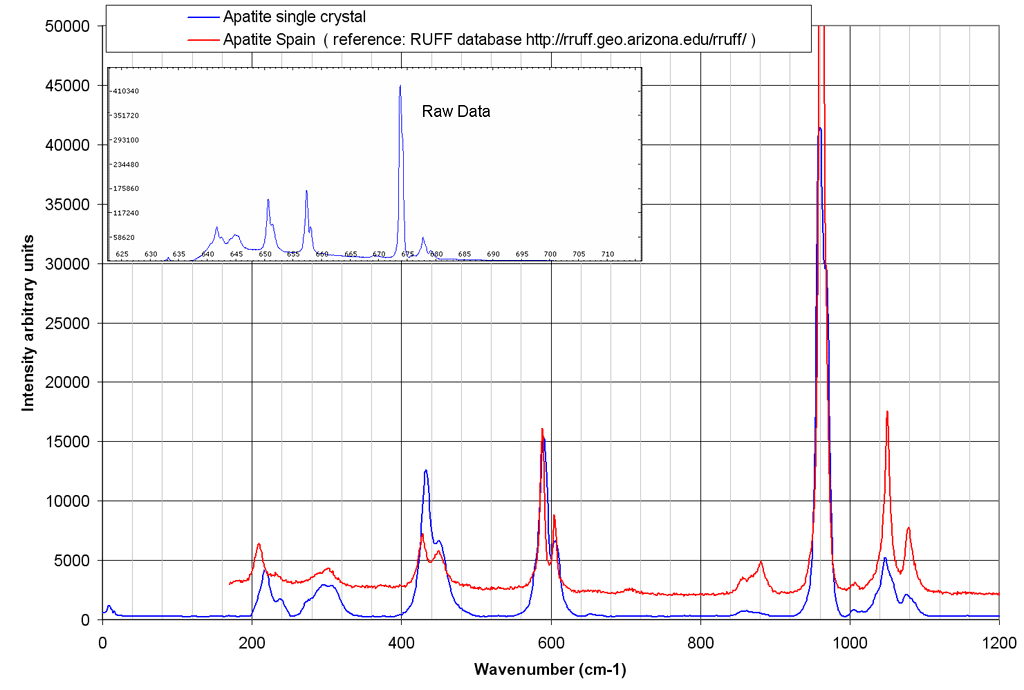
To get the final spectrum as presented here in figure 6, two additional steps must be performed: baseline correction and recalculation of the x-axis in wave numbers (cm-1). The baseline correction was performed with an old version of the Lab Control Spectacle software (1995) which allows to draw a multi points background. The recalculation of the abscissa and spectrum presentation and comparison is made in MS Excel. In order to evaluate the present Raman microscope design, I had to compare my own spectra with references from the literature. To do that, I used extensively the Database of Raman spectroscopy, X-ray diffraction and chemistry of minerals (http://rruff.geo.arizona.edu/rruff/) ( see Bibliography for complete reference). The apatite spectrum obtained with the described microscope is similar to the data of the literature except the relative intensities of the peaks as mentioned above. My spectra always have higher intensities in the low wave numbers range and lower intensities around 1000 cm-1. Nevertheless, the spectra from the present work can be used for the identification of the minerals.
|


Previous page Next Page Raman Main Page